Ansys solution example
This example shows how you can create a simple geometry directly using pansys, apply boundary conditions, loads, materials etc and run the solution.
In [1]:
from pansys import Ansys
In [2]:
ans = Ansys(startcommand='ansys150 -p ansys', cleanup=True)
In [3]:
ans.send('/prep7')
Creating the FE model
In [4]:
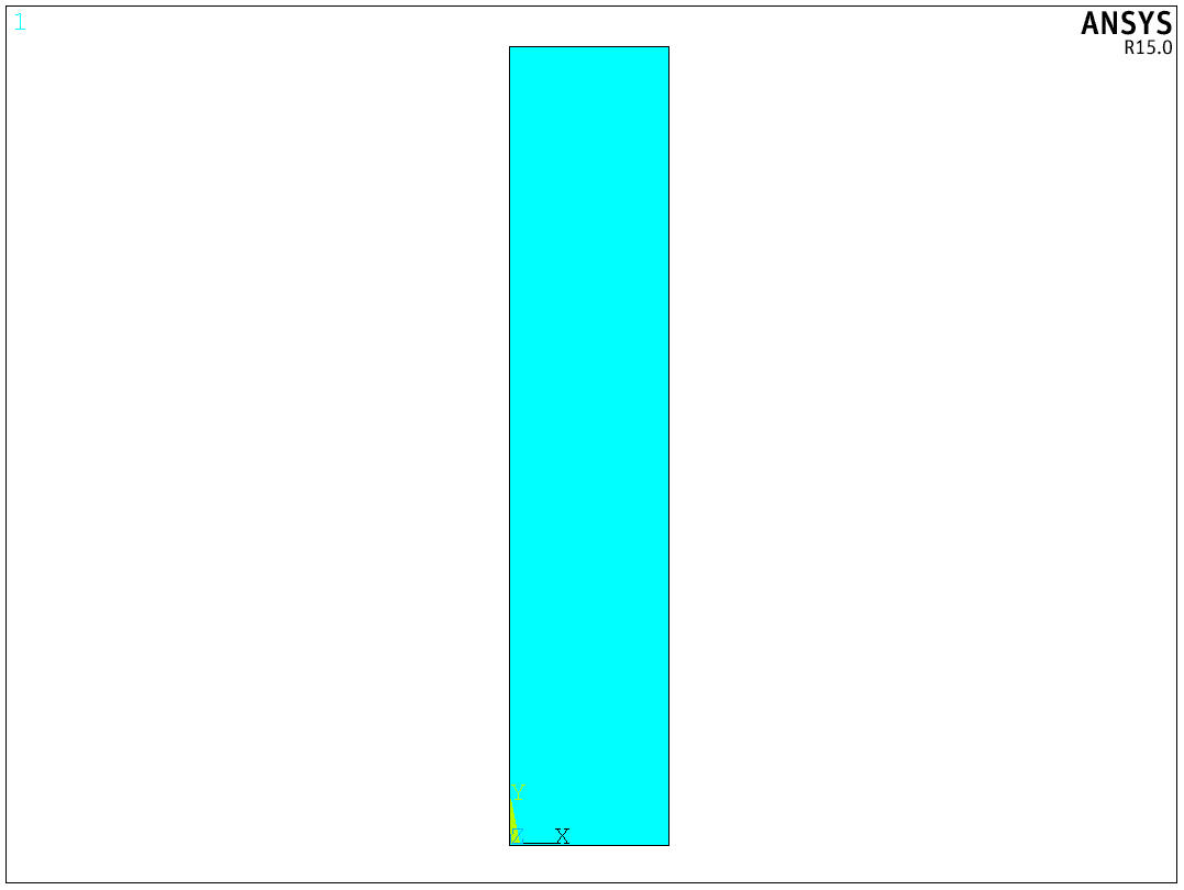
ans.send('block,0,1,0,5,0,10,')
In [5]:
img = ans.plot('aplot')
In [6]:
from IPython.display import Image
In [7]:
Image(img)
Out[7]:
In [8]:
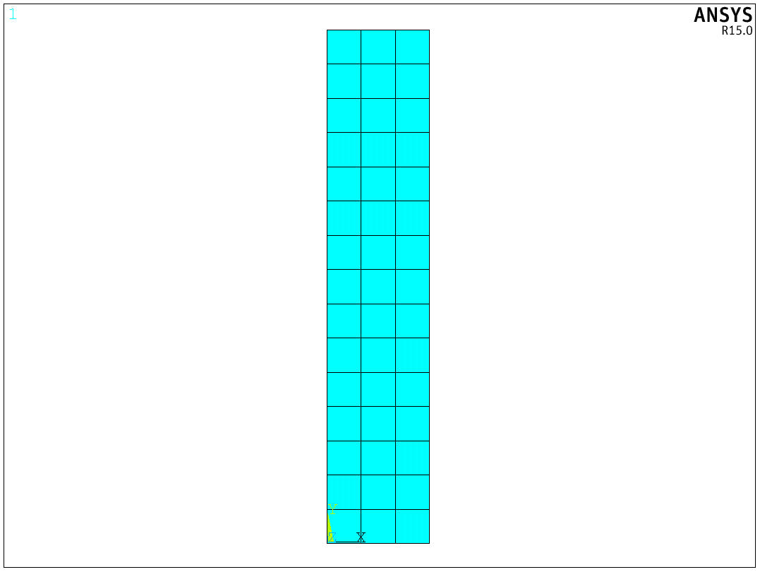
ans.send("et,1,SOLID185")
In [9]:
ans.send("vsweep, all")
In [10]:
Image(ans.plot('eplot'))
Out[10]:
Creating components boundary conditions and loads
In [11]:
ans.send('nsel,r,loc,z,-0.01,0.01')
In [12]:
ans.send('cm,fixity,node')
In [13]:
ans.send('nsel,s,loc,z,10-0.01,10+0.01')
In [14]:
ans.send('cm,load,node')
Applying loads and boundary conditions
In [15]:
nnodes = ans.get('node','','count')
In [16]:
nnodes
Out[16]:
64
In [17]:
load_val = 1000
In [18]:
ans.send("""
finish
/solu
""")
In [19]:
ans.send("""
cmsel,s,fixity
d,all,all
""")
In [20]:
ans.send("""
cmsel,s,load
f,all,fx,{}
""".format(load_val/nnodes))
In [21]:
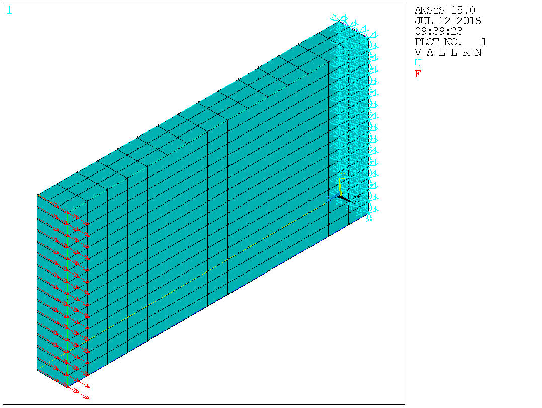
ans.send("allsel")
In [22]:
ans.send("""
/view,1,1,1,1
/ang,1
/auto,1
""")
In [23]:
ans.send('/pbc,all,,1')
In [24]:
Image(ans.plot('gplot'))
Out[24]:
Start solution
After issueing the solve command, Ansys may show some warnings and ask whether it you want to proceed or not. pansys always asks ansys to proceed. The assumption here is that pansys is not really a replacement for interactive ANSYS, instead its a means to perform complicated automations with ANSYS. Hence, the user already know what she/he is going to do.
Setting the silent key of send command to False will make
pansys show the output of the command in real time. If you want to
process the output yourselves, you can pass a function to send
command with output_func keyword argument.
In [27]:
ans.send('solve', silent=False)
solve

*****  ANSYS SOLVE    COMMAND  *****
*** NOTE ***                            CP =       0.838   TIME= 09:39:23
There is no title defined for this analysis.
*** SELECTION OF ELEMENT TECHNOLOGIES FOR APPLICABLE ELEMENTS ***
                ---GIVE SUGGESTIONS ONLY---

 ELEMENT TYPE    1 IS SOLID185. IT IS ASSOCIATED WITH LINEAR MATERIALS ONLY
 AND POISSON'S RATIO IS NOT GREATER THAN 0.49. KEYOPT(2)=3 IS SUGGESTED.


                       S O L U T I O N   O P T I O N S

   PROBLEM DIMENSIONALITY. . . . . . . . . . . . .3-D
   DEGREES OF FREEDOM. . . . . . UX   UY   UZ
   ANALYSIS TYPE . . . . . . . . . . . . . . . . .STATIC (STEADY-STATE)
   GLOBALLY ASSEMBLED MATRIX . . . . . . . . . . .SYMMETRIC

 *** WARNING ***                         CP =       0.844   TIME= 09:39:23
 Element 1 (SOLID185) uses material 1 for which Poisson's ratio is
 undefined.  A default value of 0.3 will be used.  Input MP,PRXY, 1,0.3
 to eliminate this warning.

 *** NOTE ***                            CP =       0.846   TIME= 09:39:23
 Present time 0 is less than or equal to the previous time.  Time will
default to 1.
*** NOTE ***                            CP =       0.846   TIME= 09:39:23
 The step data was checked and warning messages were found.
  Please review output or errors file (
 /home/yy53393/github/pansys/docs/_src/examples/pansys_20180712093919/fi
 ile.err ) for these warning messages.

 *** NOTE ***                            CP =       0.846   TIME= 09:39:23
 Results printout suppressed for interactive execute.

 *** NOTE ***                            CP =       0.846   TIME= 09:39:23
 The conditions for direct assembly have been met.  No .emat or .erot
 files will be produced.

 *** WARNING ***                         CP =       0.846   TIME= 09:39:23
 A check of your load data produced 1 warnings.
Should the SOLV command be executed? [y/n]
y
L O A D   S T E P   O P T I O N S

   LOAD STEP NUMBER. . . . . . . . . . . . . . . .     1
   TIME AT END OF THE LOAD STEP. . . . . . . . . .  1.0000
   NUMBER OF SUBSTEPS. . . . . . . . . . . . . . .     1
   STEP CHANGE BOUNDARY CONDITIONS . . . . . . . .    NO
   PRINT OUTPUT CONTROLS . . . . . . . . . . . . .NO PRINTOUT
   DATABASE OUTPUT CONTROLS. . . . . . . . . . . .ALL DATA WRITTEN
FOR THE LAST SUBSTEP

SOLUTION MONITORING INFO IS WRITTEN TO FILE= file.mntr

Range of element maximum matrix coefficients in global coordinates
 Maximum = 1.083214625E+10 at element 398.
 Minimum = 1.083214625E+10 at element 595.

   *** ELEMENT MATRIX FORMULATION TIMES
  TYPE    NUMBER   ENAME      TOTAL CP  AVE CP

     1       675  SOLID185      0.119   0.000176
Time at end of element matrix formulation CP = 1.12382901.
SPARSE MATRIX DIRECT SOLVER.
Number of equations =        2880,    Maximum wavefront =     60
Memory allocated for solver =                 15.259 MB
  Memory required for in-core =                  6.777 MB
  Optimal memory required for out-of-core =      2.017 MB
  Minimum memory required for out-of-core =      1.608 MB

 *** NOTE ***                            CP =       1.306   TIME= 09:39:26
 The Sparse Matrix solver is currently running in the in-core memory
 mode.  This memory mode uses the most amount of memory in order to
 avoid using the hard drive as much as possible, which most often
 results in the fastest solution time.  This mode is recommended if
 enough physical memory is present to accommodate all of the solver
data.
curEqn=   2881  totEqn=   2880 Job CP sec=      1.150
Factor Done= 100% Factor Wall sec=      0.053 rate=    1553.7 Mflops
Sparse solver maximum pivot= 8.359709376E+10 at node 739 UY.
 Sparse solver minimum pivot= 5.27830482E+09 at node 564 UX.
 Sparse solver minimum pivot in absolute value= 5.27830482E+09 at node
564 UX.
*** ELEMENT RESULT CALCULATION TIMES
  TYPE    NUMBER   ENAME      TOTAL CP  AVE CP

     1       675  SOLID185      0.135   0.000200

   *** NODAL LOAD CALCULATION TIMES
  TYPE    NUMBER   ENAME      TOTAL CP  AVE CP

     1       675  SOLID185      0.012   0.000018
 *** LOAD STEP     1   SUBSTEP     1  COMPLETED.    CUM ITER =      1
*** TIME =   1.00000         TIME INC =   1.00000      NEW TRIANG MATRIX


*** ANSYS BINARY FILE STATISTICS
BUFFER SIZE USED= 16384
1.000 MB WRITTEN ON ASSEMBLED MATRIX FILE: file.full
1.500 MB WRITTEN ON RESULTS FILE: file.rst

SOLU_LS2:
In [29]:
ans.send("""
finish
/post1""")
Post processing
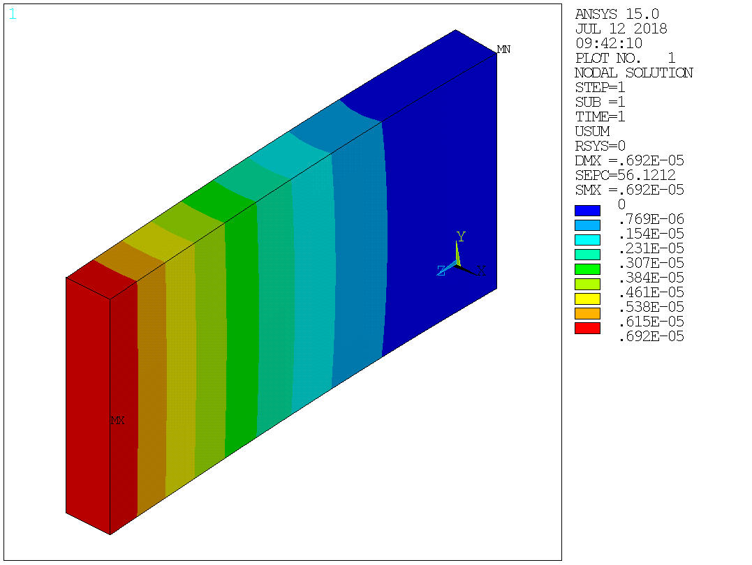
You can directly make plots from a Jupyter-notebook using the Image
method of IPython.display module and plot method of Ansys
object.
Any plotting command passed to plot function will produce a new
image file and return the path to that image file.
In [30]:
Image(ans.plot('plnsol,u,sum'))
Out[30]:
Extracting lists
Using the get_list method, you can extract any list which will
return data in a column format. The function internally uses
pandas.read_table and passes all keyword arguments from get_list
to pandas.read_table. Hence, you can use your own settings in case
need arises.
In the following section, the displacement values from result is
extracted and added it to the original coordinates of the nodes to get
the updated positions. You can pass this back to the model to by writing
out this dataframe and reading it back into model using nread
command in ANSYS.
Extract displacements
In [31]:
disp = ans.get_list('prnsol,u,sum')
Setting node numbers as the index of the dataframe.
In [35]:
disp = disp.set_index('NODE')
In [41]:
disp.head()
Out[41]:
| UX | UY | UZ | USUM | |
|---|---|---|---|---|
| NODE | ||||
| 1 | 4.175461e-08 | 1.795474e-08 | 5.657464e-08 | 7.257073e-08 |
| 2 | 1.556826e-07 | 2.465593e-08 | 1.200923e-07 | 1.981594e-07 |
| 3 | 3.574027e-07 | 2.815715e-08 | 1.785558e-07 | 4.005142e-07 |
| 4 | 6.338732e-07 | 2.988743e-08 | 2.333957e-07 | 6.761376e-07 |
| 5 | 9.814102e-07 | 2.976412e-08 | 2.831793e-07 | 1.021882e-06 |
Getting the nodal locations
In [33]:
nlocs = ans.get_list('nlist')
In [38]:
nlocs = nlocs.set_index("NODE")
In [42]:
nlocs.head()
Out[42]:
| X | Y | Z | THXY | THYZ | THZX | |
|---|---|---|---|---|---|---|
| NODE | ||||||
| 1 | 0.0 | 0.33333 | 0.66667 | 0.0 | 0.0 | 0.0 |
| 2 | 0.0 | 0.33333 | 1.33330 | 0.0 | 0.0 | 0.0 |
| 3 | 0.0 | 0.33333 | 2.00000 | 0.0 | 0.0 | 0.0 |
| 4 | 0.0 | 0.33333 | 2.66670 | 0.0 | 0.0 | 0.0 |
| 5 | 0.0 | 0.33333 | 3.33330 | 0.0 | 0.0 | 0.0 |
Creating a copy of nodal location dataframe and modifiying its X,Y and Z values to reflect the displacement results.
In [43]:
newloc = nlocs.copy()
In [47]:
newloc.X = newloc.X + disp.UX
newloc.Y = newloc.X + disp.UY
newloc.Z = newloc.X + disp.UZ
In [48]:
newloc.head()
Out[48]:
| X | Y | Z | THXY | THYZ | THZX | |
|---|---|---|---|---|---|---|
| NODE | ||||||
| 1 | 1.670184e-07 | 1.849732e-07 | 2.235931e-07 | 0.0 | 0.0 | 0.0 |
| 2 | 6.227303e-07 | 6.473862e-07 | 7.428226e-07 | 0.0 | 0.0 | 0.0 |
| 3 | 1.429611e-06 | 1.457768e-06 | 1.608166e-06 | 0.0 | 0.0 | 0.0 |
| 4 | 2.535493e-06 | 2.565380e-06 | 2.768889e-06 | 0.0 | 0.0 | 0.0 |
| 5 | 3.925641e-06 | 3.955405e-06 | 4.208820e-06 | 0.0 | 0.0 | 0.0 |
Extracting stress results
prnsol,s,prin will output the principal stresses, stress intensity
and equivalent stress as a column data. This when passed to get_list
command will create a pandas DataFrame object which you can do
operations on.
In [49]:
stress = ans.get_list('prnsol,s,prin')
In [57]:
stress_comp = ans.get_list('prnsol,s,comp')
In [51]:
stress.describe()
Out[51]:
| NODE | S1 | S2 | S3 | SINT | SEQV | |
|---|---|---|---|---|---|---|
| count | 1024.00000 | 1024.000000 | 1.024000e+03 | 1024.000000 | 1024.000000 | 1024.000000 |
| mean | 512.50000 | 1759.415595 | 3.906240e-10 | -1759.415595 | 3518.831191 | 3373.138197 |
| std | 295.74764 | 2360.955818 | 4.121431e+02 | 2360.955818 | 2755.911176 | 2638.761378 |
| min | 1.00000 | -67.431017 | -1.516078e+03 | -10182.646000 | 249.533180 | 232.421030 |
| 25% | 256.75000 | 195.068432 | -2.051532e+02 | -2523.917175 | 1414.674325 | 1362.514750 |
| 50% | 512.50000 | 555.387185 | 0.000000e+00 | -555.387185 | 2718.112550 | 2668.931550 |
| 75% | 768.25000 | 2523.917175 | 2.051532e+02 | -195.068432 | 5313.088775 | 5205.215950 |
| max | 1024.00000 | 10182.646000 | 1.516078e+03 | 67.431017 | 10396.160000 | 9738.712700 |
In [58]:
stress_comp.describe()
Out[58]:
| NODE | SX | SY | SZ | SXY | SYZ | SXZ | |
|---|---|---|---|---|---|---|---|
| count | 1024.00000 | 1.024000e+03 | 1.024000e+03 | 1.024000e+03 | 1.024000e+03 | 1.024000e+03 | 1024.000000 |
| mean | 512.50000 | -9.768519e-12 | -4.440892e-16 | -1.012523e-13 | -4.462516e-11 | -9.960925e-10 | 261.900917 |
| std | 295.74764 | 3.877772e+02 | 4.235339e+02 | 4.016076e+03 | 7.717880e+01 | 2.005821e+02 | 643.002914 |
| min | 1.00000 | -1.197029e+03 | -1.516337e+03 | -9.184036e+03 | -5.706479e+02 | -1.523964e+03 | -766.467980 |
| 25% | 256.75000 | -9.239690e+01 | -2.432290e+02 | -2.510376e+03 | -8.206400e+00 | -5.648059e+01 | 48.175390 |
| 50% | 512.50000 | 0.000000e+00 | 0.000000e+00 | 0.000000e+00 | 6.068757e-14 | -5.000000e-09 | 112.944940 |
| 75% | 768.25000 | 9.239690e+01 | 2.432290e+02 | 2.510376e+03 | 8.206400e+00 | 5.648059e+01 | 166.714970 |
| max | 1024.00000 | 1.197029e+03 | 1.516337e+03 | 9.184036e+03 | 5.706479e+02 | 1.523964e+03 | 3476.179700 |
In [56]:
stress[stress.SEQV == stress.SEQV.max()]
Out[56]:
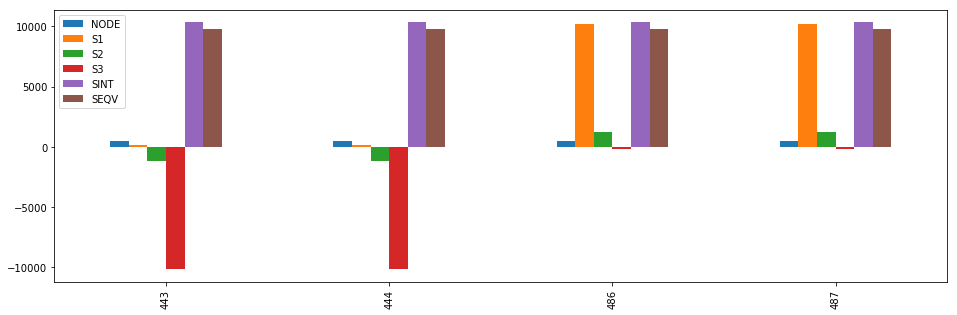
| NODE | S1 | S2 | S3 | SINT | SEQV | |
|---|---|---|---|---|---|---|
| 443 | 444 | 157.91667 | -1185.212 | -10182.64600 | 10340.563 | 9738.7127 |
| 444 | 445 | 157.91667 | -1185.212 | -10182.64600 | 10340.563 | 9738.7127 |
| 486 | 487 | 10182.64600 | 1185.212 | -157.91667 | 10340.563 | 9738.7127 |
| 487 | 488 | 10182.64600 | 1185.212 | -157.91667 | 10340.563 | 9738.7127 |
Plotting stress results
In [66]:
%matplotlib inline
In [68]:
stress[stress.SEQV == stress.SEQV.max()].plot(kind='bar', figsize=(16,5))
Out[68]:
<matplotlib.axes._subplots.AxesSubplot at 0x7fc7cc6d2080>
Finding the stress components of nodes with high equivalent stress
The following commands will extract all nodes where stress is equal to or greater than 95% of max equivalent stress and show their component stresses.
In [70]:
eqv_nodes = stress[stress.SEQV >= stress.SEQV.max()].NODE.values
stress_comp[stress_comp.NODE.apply(lambda x: x in eqv_nodes)]
Out[70]:
| NODE | SX | SY | SZ | SXY | SYZ | SXZ | |
|---|---|---|---|---|---|---|---|
| 443 | 444 | -1185.212 | -1185.212 | -8839.5173 | -2.768785e-12 | -29.764415 | 3476.1797 |
| 444 | 445 | -1185.212 | -1185.212 | -8839.5173 | 3.013895e-12 | 29.764415 | 3476.1797 |
| 486 | 487 | 1185.212 | 1185.212 | 8839.5173 | 2.440367e-12 | -29.764415 | 3476.1797 |
| 487 | 488 | 1185.212 | 1185.212 | 8839.5173 | -2.427766e-12 | 29.764415 | 3476.1797 |
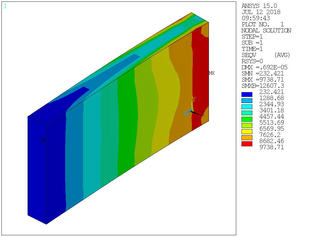
In [53]:
Image(ans.plot('plnsol,s,eqv'))
Out[53]:
In [ ]: